Lab 7: Kalman Filter

The purpose of this lab is to implement a Kalman Filter to supplement the slowly-updating ToF sensor with a faster state estimate, allowing the PID controller to run at a higher effective rate. The VL53L1X ToF sensor is limited to ~10–20 Hz in practice, but the Artemis control loop runs much faster. The Kalman Filter predicts the car's position and velocity at every loop iteration using a state-space model of the car's dynamics, and corrects that estimate each time a new ToF reading arrives. This way, the PID controller always has a fresh, smooth position estimate to work with, even between sensor updates.

To build the state-space model, I need to estimate the drag coefficient d and momentum term m. These come directly from a step response experiment: drive the car toward a wall at a constant PWM input and observe how speed evolves over time.

Step Response Setup

I chose u = 150 PWM as the step input, which is approximately 59% of the maximum PWM (255) and consistent with the PWM used in Lab 5, keeping the dynamics comparable. I placed the car roughly 4 feet from the wall with a foam cushion as a buffer. The ToF sensor was set to short-distance mode for a higher sampling rate (~20 Hz), and the control loop was made non-blocking so the Artemis logs data as fast as sensor readings arrive rather than blocking on each measurement.

The step response Arduino code drives the car at a constant PWM, takes non-blocking ToF readings, and auto-brakes when the car gets within STOP_DISTANCE of the wall:

void runStepResponse() {
    if (sensor2.checkForDataReady()) {
        distance2 = sensor2.getDistance();
        sensor2.clearInterrupt();
        sensor2.stopRanging();
        sensor2.startRanging();
 
        if (distance2 < STOP_DISTANCE) {
            stop();
            step_running = false;
            return;
        }
 
        if (arr_index < ARRAY_SIZE) {
            T_arr[arr_index]                 = millis();
            Measured_distance_arr[arr_index] = distance2;
            Control_speed_arr[arr_index]     = STEP_PWM;
            arr_index++;
        }
    }
    forward(STEP_PWM);
}

On the Python side, data is collected over BLE and saved immediately to a pickle file so it persists across kernel restarts:

data = {"T": T_arr, "D": Distance_arr, "U": MotorInput_arr}
with open("step_response.pkl", "wb") as f:
    pickle.dump(data, f)
 
# Load back after restart:
with open("step_response.pkl", "rb") as f:
    data = pickle.load(f)
T_arr, Distance_arr, MotorInput_arr = data["T"], data["D"], data["U"]

Initial Attempt: Long Distance Mode (141 inches)

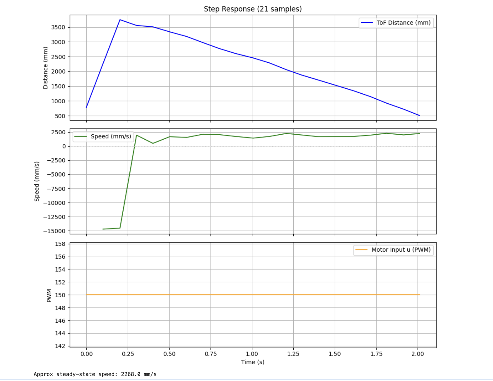
My first attempt started 141 inches from the wall using long-distance ToF mode. The sensor produced a large distance spike at the start (an unstable reading before the sensor stabilized), and long-distance mode is limited to ~10 Hz, so only 21 samples were collected over 2 seconds. The speed curve plateaued almost immediately, suggesting the car reached steady state faster than the sensor could capture the ramp-up.

Step Response Video

Step Response Graphs

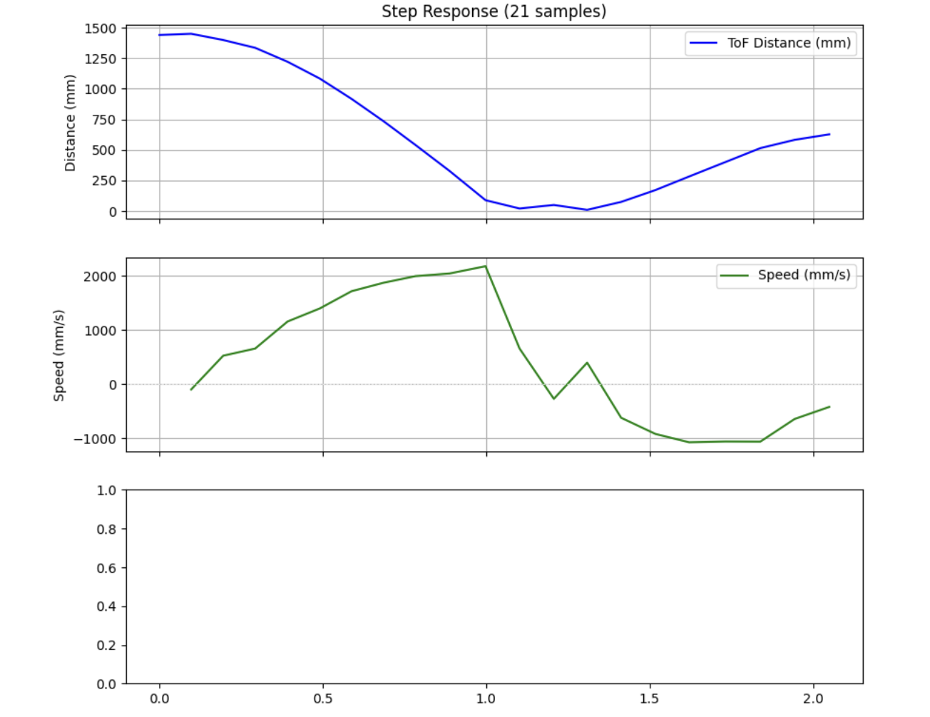
The computed speed is derived from the ToF distance data as: speed = -ΔDistance / Δtime (negated because distance decreases as the car moves forward). The motor input is a constant horizontal line at 150 PWM — this is the step input u(t) that the car's dynamics respond to.

The speed curve clearly shows the car accelerating from rest and approaching a plateau, consistent with a first-order system reaching terminal velocity where motor force balances drag. My car hit the foam buffer at approximately the 10th sample, so only the first 10 samples (indices 0–9) are used for extracting steady-state speed.

Extracting d and m

From the pre-crash portion of the speed data, I extracted the three key values needed:

speed_clean = speed[:10]
T_clean     = T_speed[:10]
 
v_ss = np.mean(speed_clean[6:10])
u    = 150
 
d = u / v_ss
 
v_90   = 0.9 * v_ss
idx_90 = np.argmax(speed_clean >= v_90)
t_90   = T_clean[idx_90]
 
m = -d * t_90 / np.log(1 - 0.9)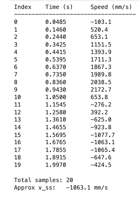

The resulting values are:

• Steady-state speed v_ss = 2017.1 mm/s — the plateau speed where motor force exactly balances drag
• 90% rise time t_90% = 0.6370 s — the time at which speed reaches 90% of v_ss
• Speed at 90% rise time v_90% = 1815.4 mm/s
• d = u / v_ss = 150 / 2017.1 = 0.0744
• m = −d · t_90% / ln(1 − 0.9) = 0.0206

As a sanity check: the velocity decay time constant is m/d = 0.0206/0.0744 ≈ 0.277 s, meaning if the motors were cut, speed would decay with a ~0.28 s time constant. This is physically reasonable for a small lightweight RC car.

State-Space Model

The car's equation of motion is m&ddot;x; = u − d˙x;, which rearranges to &ddot;x; = −(d/m)˙x; + (1/m)u. With state vector x = [position, velocity]^T, the continuous-time state-space matrices are:

A = np.array([[0,    1  ],
              [0,  -d/m ]])   # system dynamics: how state evolves on its own
 
B = np.array([[0  ],
              [1/m]])          # input matrix: how PWM affects state

Discretization

The total step response run time was approximately 2 seconds with 21 samples, giving an inter-sample interval of about 0.095 s. I use ΔT = 0.1 s as the sampling time. Discretization uses the first-order Euler approximation: A_d = I + ΔT·A and B_d = ΔT·B.

Delta_T = 0.1
n = 2
Ad = np.eye(n) + Delta_T * A
Bd = Delta_T * B

C Matrix

The measurement matrix C maps the full state vector to what the ToF sensor can actually observe. The ToF measures positive distance, but the state convention defines position as negative distance from the wall (car moving toward wall is positive). C = [−1, 0] flips the sign to match: y = Cx = −position = +distance. The zero in the second column reflects that velocity is never directly measured — the Kalman Filter must estimate it.

C = np.array([[-1, 0]])

State Initialization and Noise Covariance

TOF = np.array(Distance_arr)
x   = np.array([[-TOF[0]], [0]])   # [negative distance, 0 velocity]
 
sigma_1 = 20    # process noise: position uncertainty (mm)
sigma_2 = 20    # process noise: velocity uncertainty (mm/s)
sigma_3 = 20    # sensor noise: ToF measurement noise (mm)
 
Sigma_u = np.array([[sigma_1**2, 0         ],
                     [0,          sigma_2**2]])
 
Sigma_z = np.array([[sigma_3**2]])

Kalman Filter Function

def kf(mu, sigma, u, y):
    mu_p    = Ad.dot(mu) + Bd.dot(u)
    sigma_p = Ad.dot(sigma.dot(Ad.T)) + Sigma_u
 
    sigma_m = C.dot(sigma_p.dot(C.T)) + Sigma_z
    kf_gain = sigma_p.dot(C.T.dot(np.linalg.inv(sigma_m)))
 
    y_m   = y - C.dot(mu_p)
    mu    = mu_p + kf_gain.dot(y_m)
    sigma = (np.eye(n) - kf_gain.dot(C)).dot(sigma_p)
 
    return mu, sigma

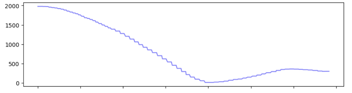
Before deploying to the Artemis, I tested the Kalman Filter in Python by running it on the previously collected Lab 5 PID data. The filter runs on the raw ToF readings offline, and the KF estimate is overlaid on the raw distance for comparison:

mu    = np.array([[-D[0]], [0]])
sigma = np.eye(n)
kf_positions = []
 
for i in range(len(D)):
    y         = np.array([[-D[i]]])
    mu, sigma = kf(mu, sigma, u_k, y)
    kf_positions.append(-mu[0, 0])

The KF output (purple) is smoother than the raw ToF (blue) while still tracking the same trajectory — confirming the filter parameters and sign conventions are correct before moving to the Artemis.

The Kalman Filter is implemented on the Artemis using the BasicLinearAlgebra library. Unlike the offline Python test, the filter now runs in real-time: the predict step executes every control loop iteration (fast), while the update step only runs when a new ToF reading is available (slow, ~20 Hz). This lets the PID controller use a continuously-updated state estimate between sensor readings rather than waiting for the next ToF sample.

KF Predict and Update (Arduino)

void kf_predict(float u_pwm) {
    unsigned long now = millis();
    float dt = (now - last_predict_time) / 1000.0f;
    last_predict_time = now;
    if (dt <= 0 || dt > 0.5) return;
 
    Matrix<2,2> Ad = {1,      dt,
                       0, 1 - (D_DRAG/M_MOM)*dt};
    Matrix<2,1> Bd = {0, dt/M_MOM};
 
    mu    = Ad * mu + Bd * u_pwm;
    Sigma = Ad * Sigma * ~Ad + Sigma_u;
}
 
void kf_update(float tof_mm) {
    Matrix<1,1> y_m     = {-tof_mm};
    Matrix<1,1> sigma_m = C_mat * Sigma * ~C_mat + Sigma_z;
    Matrix<2,1> kf_gain = Sigma * ~C_mat * Inverse(sigma_m);
 
    mu = mu + kf_gain * (y_m - C_mat * mu);
 
    Matrix<2,2> I_mat = {1, 0, 0, 1};
    Sigma = (I_mat - kf_gain * C_mat) * Sigma;
}
 
float kf_distance() {
    return -mu(0, 0);
}

KF + PID Control Loop

void runKFPIDController() {
    kf_predict((float)abs(linear_control_speed));
 
    if (sensor2.checkForDataReady()) {
        distance2 = sensor2.getDistance();
        sensor2.clearInterrupt();
        sensor2.stopRanging();
        sensor2.startRanging();
 
        if (!kf_initialized) {
            mu(0, 0)          = -(float)distance2;
            mu(1, 0)          = 0;
            last_predict_time = millis();
            kf_initialized    = true;
            return;
        }
        kf_update((float)distance2);
    }
 
    if (!kf_initialized) return;
 
    float kf_dist = kf_distance();
    if (kf_dist < 0 || kf_dist > 5000) kf_dist = (float)distance2;
 
    linear_error         = (int)(kf_dist - LINEAR_SETPOINT);
    linear_sum_error    += linear_error;
    int derivative       = linear_error - linear_previous_error;
    linear_control_speed = (int)(linear_Kp*linear_error
                               + linear_Ki*linear_sum_error
                               + linear_Kd*derivative);
    linear_previous_error = linear_error;
    linear_control_speed  = constrain(abs(linear_control_speed), MIN_SPEED, MAX_SPEED);
 
    if (arr_index < ARRAY_SIZE) {
        T_arr[arr_index]                 = millis();
        Measured_distance_arr[arr_index] = distance2;
        KF_distance_arr[arr_index]       = (int)kf_dist;
        Error_arr[arr_index]             = linear_error;
        Control_speed_arr[arr_index]     = linear_control_speed;
        arr_index++;
    }
 
    if (abs(linear_error) < 20) {
        stop();
    } else if (linear_error > 0) {
        forward(linear_control_speed);
    } else {
        backward(linear_control_speed);
    }
}

Result: KF + PID at PWM 150

• Lab 6 Instructions — Fast Robots @ Cornell
• Trevor Dales's Lab 7 Report (referenced for math and some code structure)
• Grammarly writing assistance is used to fix my report's grammar and sentence flow.