Lab 3: Time of Flight Sensors
Objective
The purpose of this lab is to equip the robot with two VL53L1X time-of-flight (ToF) distance sensors. The faster the robot can sample and the more it can trust a sensor reading, the faster it is able to drive. This lab covers sensor characterization (range, accuracy, repeatability, ranging time), dual-sensor setup over I2C, non-blocking data collection, and streaming time-stamped ToF and IMU data over Bluetooth to a laptop.
Prelab
Prior to lab, I skimmed the VL53L1X API manual and the datasheet to understand the sensor's I2C interface, addressing, and ranging modes.
I2C Address
The VL53L1X has an 8-bit hardware I2C address of 0x52 (write) / 0x53 (read) per the
datasheet. The Arduino Wire library uses 7-bit addresses, so the effective address seen
in code is 0x52 >> 1 = 0x29. Both sensors share this same default
address out of the box.
Approach: Two ToF Sensors on the Same I2C Bus
Since both sensors default to address 0x29, placing them on the same I2C bus without any intervention causes address conflicts — both sensors respond simultaneously, garbling the data. There are two solutions:
-
Programmatic address change: While the sensor is powered, call
setI2CAddress()to remap one sensor to a new address. The change is stored in volatile memory and is lost on power cycle, requiring re-initialization every boot. - XSHUT pin approach: Pull one sensor's XSHUT line LOW to shut it off, initialize and remap the other sensor, then release XSHUT to wake the second sensor at its default address.
I chose the XSHUT approach because it makes the initialization sequence explicit and deterministic. On every power cycle, the boot sequence re-establishes unique addresses, so even if a sensor resets mid-operation it will be correctly re-initialized. Only Sensor 2's XSHUT is wired to Artemis pin A0; Sensor 1 is always powered and gets its address changed to 0x30 during setup.
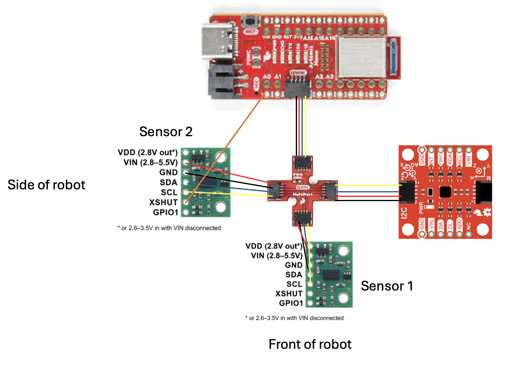
Sensor Placement on Robot
I plan to mount one sensor at the front of the robot (Sensor 1) and one on the side (Sensor 2). This gives simultaneous forward and lateral obstacle coverage: the front sensor enables forward collision avoidance, and the side sensor enables wall-following and side-clearance detection.
Scenarios where the robot will miss obstacles: obstacles that are very low to the ground (below the sensor's field of view), highly transparent or IR-absorbing surfaces (glass, dark foam), obstacles in the robot's rear quadrant, and narrow objects that fall outside the sensor's ~25° detection cone.
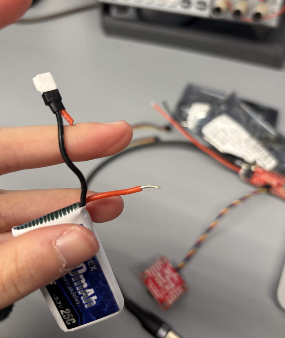
Task 1: JST Connector Battery and Powering Artemis
I soldered a JST connector to the 650 mAh battery from the RC car. The process:
- Cut one end of a Qwiic cable (one wire at a time — never both simultaneously, as this shorts the battery terminals).
- Strip, twist, and pre-tin each wire end.
- Solder and cover each joint with heat shrink tubing (not electrical tape, which can fall off and leave residue).
- Check polarity by briefly connecting to the Artemis. The JST connector color convention is not standardized — my battery's red and black were reversed relative to the Artemis connector, so I connected black-to-red and red-to-black.
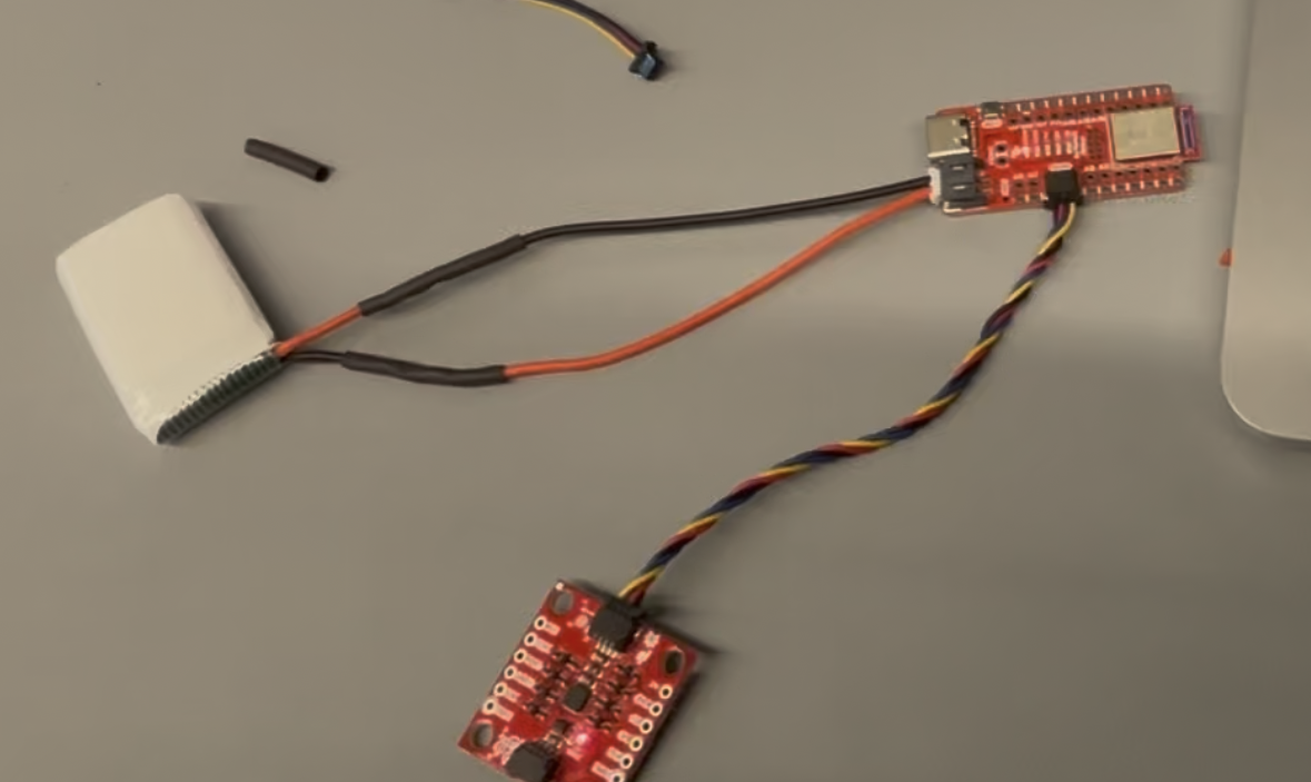
I verified the battery-powered setup by running the BLE PING/PONG test from Lab 1 with the USB disconnected. The Artemis advertised over BLE and responded correctly, confirming untethered operation. Note: the Artemis also charges the battery when USB is simultaneously connected.
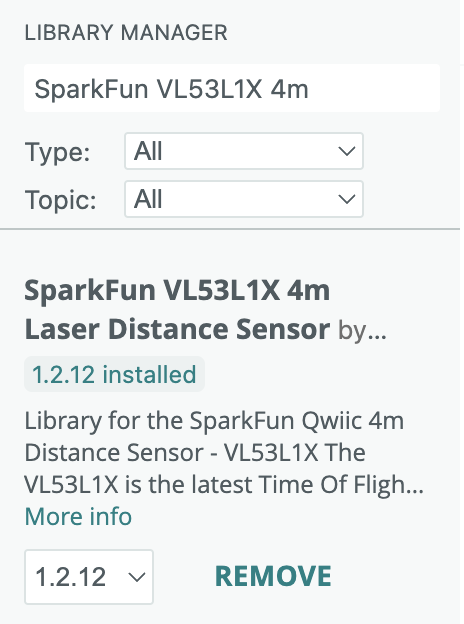
Task 2: SparkFun VL53L1X 4m Laser Distance Sensor Library
Using the Arduino Library Manager, I installed the
SparkFun VL53L1X 4m Laser Distance Sensor library (version 1.2.12).
This library provides a high-level C++ API for the VL53L1X, abstracting the ST
Microelectronics driver. It exposes the key methods used throughout this lab:
begin(), startRanging(), checkForDataReady(),
getDistance(), clearInterrupt(), stopRanging(),
setDistanceModeLong(), and setI2CAddress().
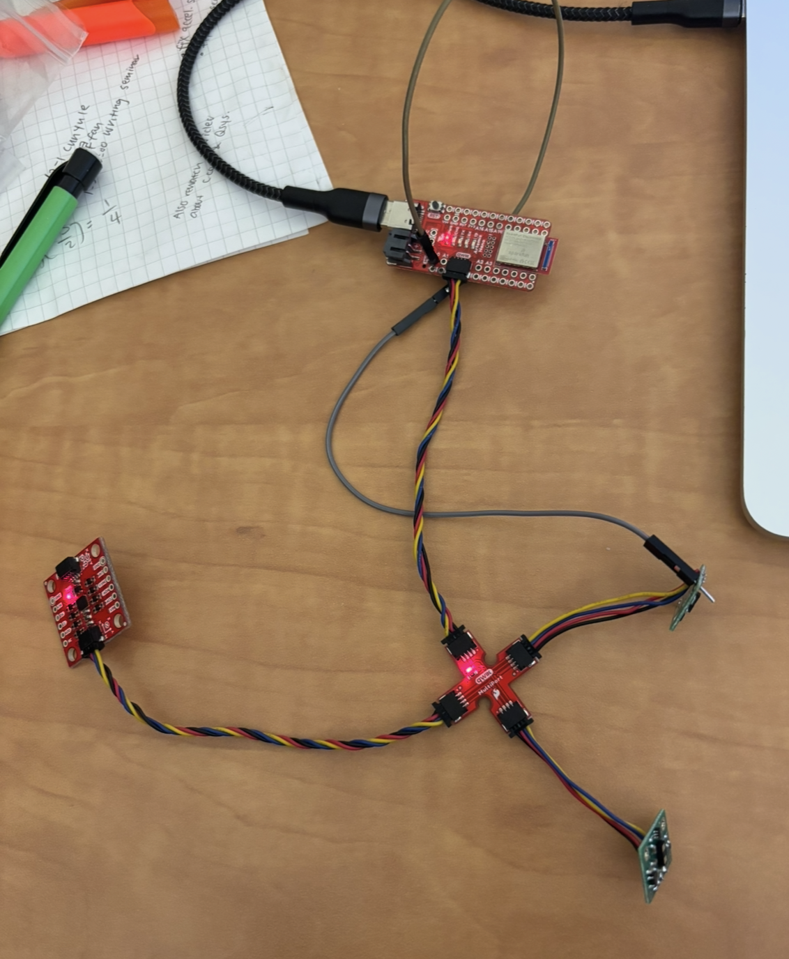
Task 3 & 4: Connect Qwiic Breakout Board and ToF Sensors
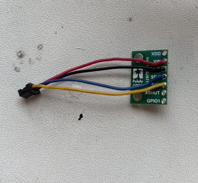
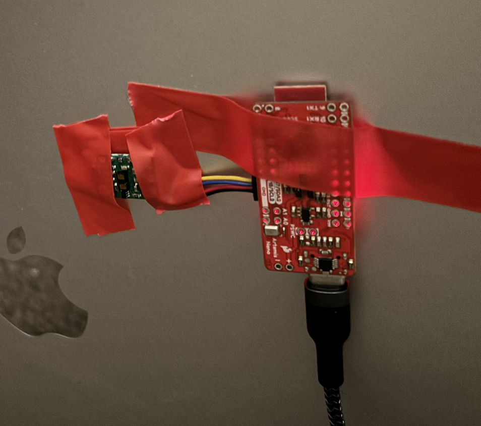
I connected the SparkFun Qwiic breakout board to the Artemis Nano using a short Qwiic cable. I then soldered long Qwiic cables to each ToF sensor breakout board, following the wire color convention:
- Blue → SDA
- Yellow → SCL
- Red → 3.3V (VIN)
- Black → GND
Long cables were used for both sensors since they will be mounted at different locations on the robot chassis and need to reach the Qwiic breakout board. Electric tape was applied to insulate the Artemis pins from shorting against the metal laptop exterior during testing.
Task 5: Scan I2C Channel (Example05_wire_I2C)
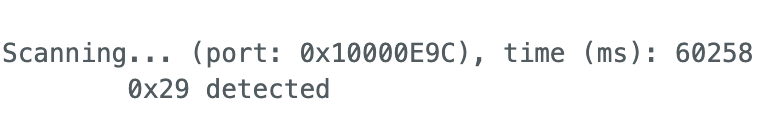
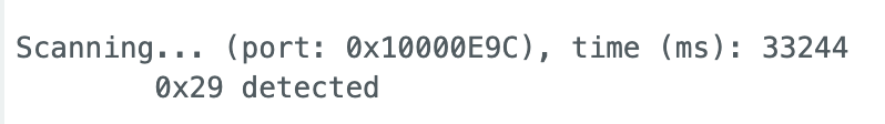
I ran File → Examples → Apollo3 → Wire → Example05_wire_I2C with each ToF sensor connected one at a time. The program iterates through 7-bit addresses 1–126 and reports which ones acknowledge an I2C transaction. Both sensors were detected at address 0x29:
Scanning... (port: 0x10000E9C), time (ms): 33244
    0x29 detected

Scanning... (port: 0x10000E9C), time (ms): 60258
    0x29 detected
At first I expected 0x52, since the VL53L1X datasheet specifies an 8-bit write
address of 0x52. However, the Wire library uses 7-bit addresses, so it scans
the range 1–126. The 8-bit address 0x52 in binary is 1010010;
right-shifting by one bit yields 101001 = 0x29. This is the
7-bit address that Wire detects and reports. Both sensors confirmed to be on
the bus at 0x29.
Task 6: Distance Modes
The VL53L1X offers three ranging modes that trade off maximum range against ambient light immunity:
| Mode | Max Distance | Pros / Cons |
|---|---|---|
| Short | Up to 1.3 m | Best ambient light immunity; limited range |
| Medium | Up to 3 m | Balanced; requires separate Pololu library |
| Long (default) | Up to 4 m | Maximum range; less immune to ambient IR noise |
I chose Long mode. The Fast Robots lab room is approximately 4 m across, and I want the maximum detection range for fast driving scenarios. The lab is well-lit indoors, so ambient IR noise is not a major concern. Long mode is also the default, requiring only an explicit confirmation call:
sensor1.setDistanceModeLong();
sensor2.setDistanceModeLong();
Note: Medium mode requires the separate Pololu VL53L1X library and is not used here.
Task 7: Test Chosen Mode — Range, Accuracy, Repeatability, Ranging Time
I tested Long mode using the SparkFun Example1_ReadDistance, then
augmented it with BLE to stream timestamped readings to Jupyter Lab for analysis.
The VL53L1X uses a 940 nm Class 1 VCSEL (Vertical Cavity Surface Emitting Laser)
to time the round-trip of an IR pulse. Per SparkFun documentation, precision is
1 mm and accuracy is approximately ±5 mm.
Setup
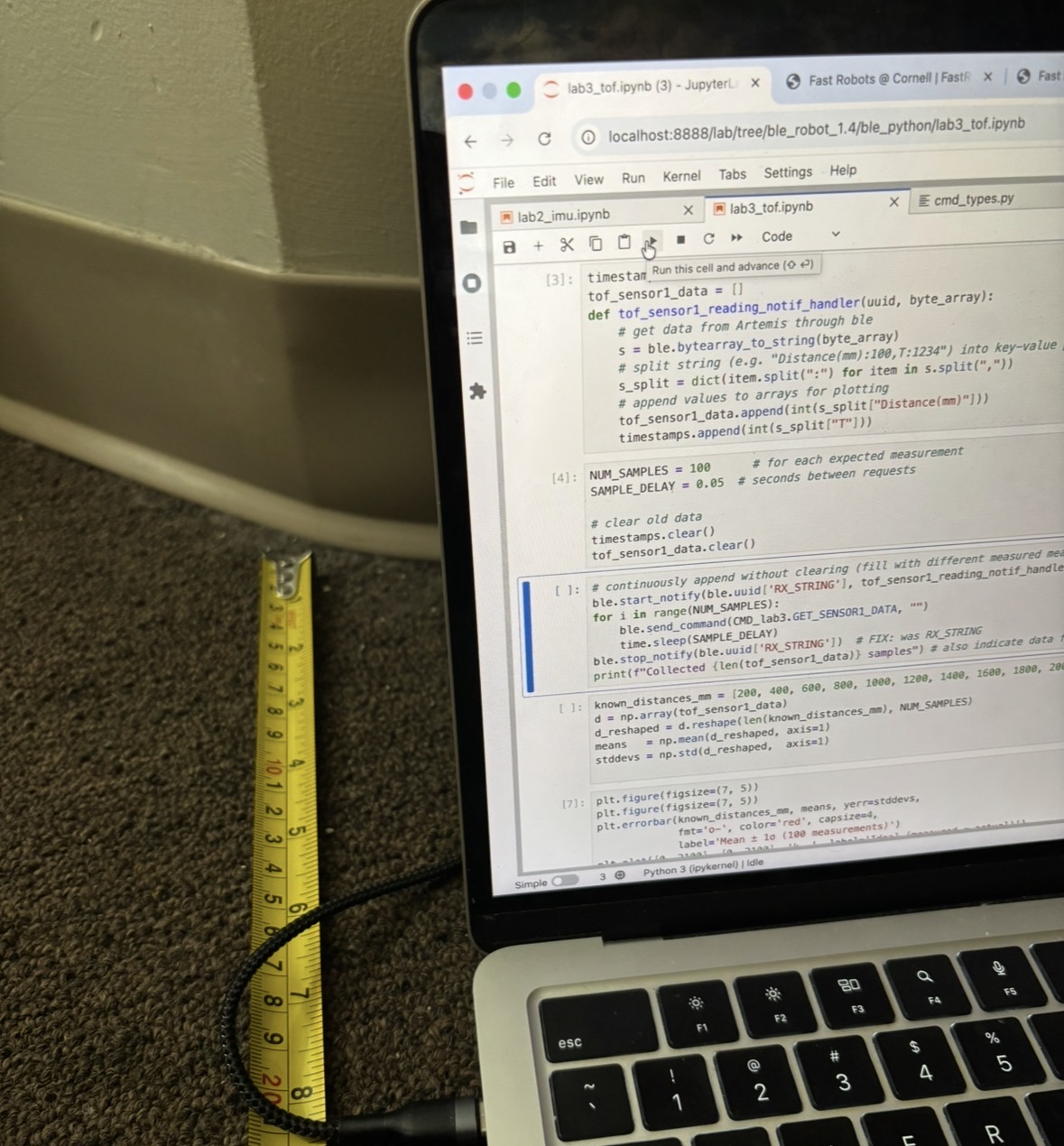
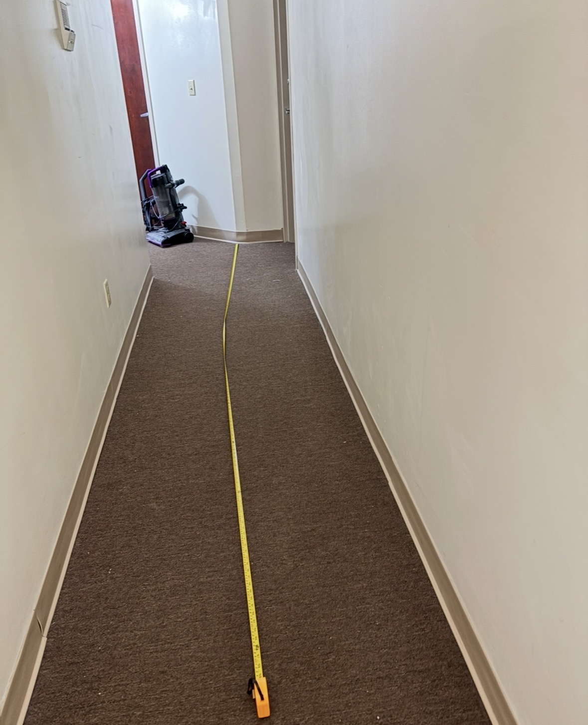
I taped the Artemis and ToF sensor to the back of my laptop (electric tape insulating the pins from the metal exterior), set up a tape measure from a wall, and moved the laptop to known distances: 200, 400, 600, 800, 1000, 1200, 1400, 1600, 1800, and 2000 mm. For each position I collected 10 samples via BLE notification, for a total of 100 measurements.
Arduino Code
// Global
int distance = 0;

// In loop(), inside while(central.connected()):
distanceSensor.startRanging();
while (!distanceSensor.checkForDataReady()) { delay(1); }
distance = distanceSensor.getDistance();
distanceSensor.clearInterrupt();
distanceSensor.stopRanging();

// On GET_SENSOR1_DATA command:
tx_estring_value.clear();
tx_estring_value.append("Distance(mm):");
tx_estring_value.append(distance);
tx_estring_value.append(",T:");
tx_estring_value.append((int)millis());
tx_characteristic_string.writeValue(tx_estring_value.c_str());
Python Collection Code
tof_data = []
def tof_notif_handler(uuid, byte_array):
    s = ble.bytearray_to_string(byte_array)
    d = dict(item.split(':') for item in s.split(','))
    tof_data.append((int(d['T']), int(d['Distance(mm)'])))

distances_mm = [200, 400, 600, 800, 1000, 1200, 1400, 1600, 1800, 2000]
means, stds = [], []

for expected in distances_mm:
    tof_data.clear()
    input(f'Move sensor to {expected}mm, then press Enter...')
    ble.start_notify(ble.uuid['TX_STRING'], tof_notif_handler)
    while len(tof_data) < 10:
        ble.send_command(CMD_lab3.GET_SENSOR1_DATA, '')
        time.sleep(0.15)
    ble.stop_notify(ble.uuid['TX_STRING'])
    vals = [d[1] for d in tof_data]
    means.append(np.mean(vals))
    stds.append(np.std(vals))
    print(f'mean={means[-1]:.1f} mm  std={stds[-1]:.1f} mm')
Results
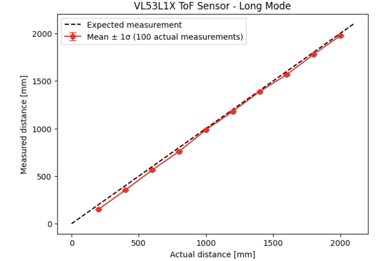
Measured mean values tracked closely with expected distances across the full 200–2000 mm range. Error bars (±1σ) were small (~3–8 mm standard deviation), indicating good repeatability consistent with the ±5 mm accuracy specification.
Troubleshooting
Several issues arose during data collection:
- All measured values initially clustered around ~300 mm regardless of expected distance — the sensor was pointing at the laptop screen instead of the wall. Fixed by tilting the laptop screen so the sensor faces the wall directly.
- Inconsistent readings due to sensor movement — fixed by taping the Artemis and sensor firmly to the back of the laptop with electric tape to insulate the pins from the metal exterior.
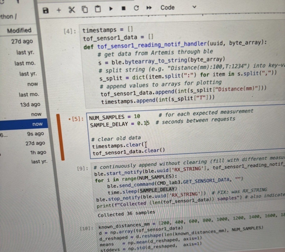
- Lost BLE samples at a sample delay of 0.05 s — fixed by increasing to 0.15 s.
- BLE disconnections during collection — reconnected and resumed.
Task 8: Hook Up Both ToF Sensors
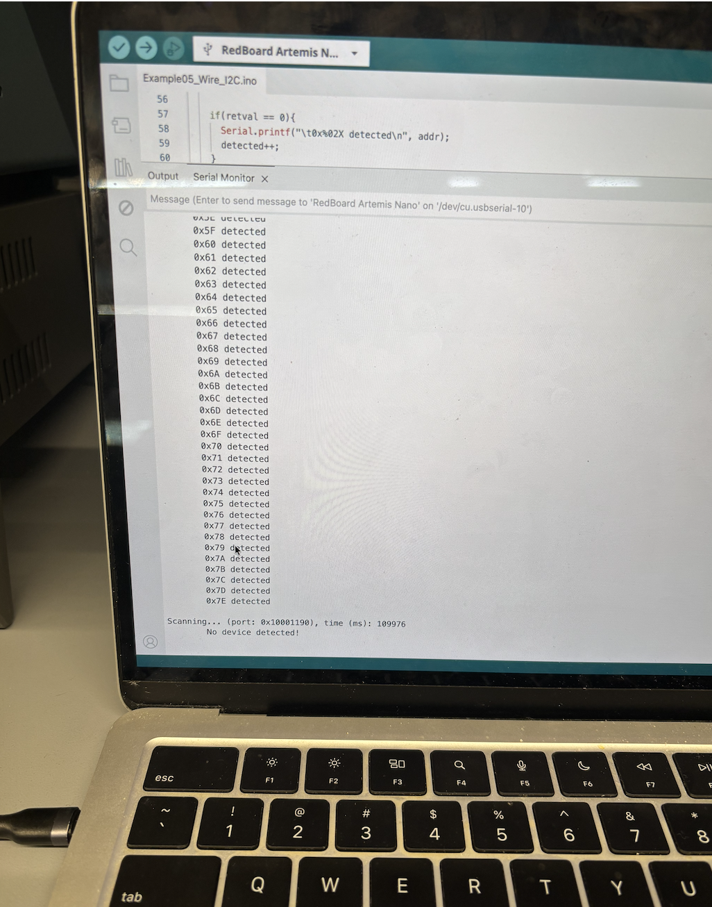
Running Example05_wire_I2C with both sensors simultaneously causes the Artemis to report a device at nearly every I2C address — both sensors pull SDA/SCL simultaneously, producing ambiguous acknowledgements. This confirms that both sensors cannot coexist at the same default address 0x29.
XSHUT Address Remapping Procedure
Only Sensor 2's XSHUT pin is wired to Artemis A0. Sensor 1 has no XSHUT wire
(always powered). The initialization sequence in setup():
- Pull A0 LOW → Sensor 2 is off. Only Sensor 1 is on the bus at 0x29.
- Call
sensor1.begin()to initialize Sensor 1. - Call
sensor1.setI2CAddress(0x30)to remap Sensor 1 (volatile memory). - Pull A0 HIGH → Sensor 2 wakes at its default address 0x29. No conflict.
- Call
sensor2.begin()to initialize Sensor 2 at 0x29.
The address change is stored in volatile memory — a power cycle requires repeating this sequence.
#define XSHUT_Sensor2 A0
SFEVL53L1X sensor1;  // remapped to 0x30
SFEVL53L1X sensor2;  // stays at 0x29

// In setup():
pinMode(XSHUT_Sensor2, OUTPUT);
digitalWrite(XSHUT_Sensor2, LOW);  // sensor 2 off
delay(50);

if (sensor1.begin() != 0) { while (1); }  // freeze on failure
sensor1.setI2CAddress(0x30);
Serial.println("Sensor 1 online at 0x30");

digitalWrite(XSHUT_Sensor2, HIGH);  // sensor 2 wakes at 0x29
delay(50);

if (sensor2.begin() != 0) { while (1); }
Serial.println("Sensor 2 online at 0x29");

sensor1.setDistanceModeLong();
sensor2.setDistanceModeLong();
The Serial Monitor confirms both sensors initialized correctly:
VL53L1X Qwiic Test
Advertising BLE with MAC: c0:81:b4:24:2b:64
Sensor 1 at 0x30
Sensor 2 at 0x29
Both sensors ready!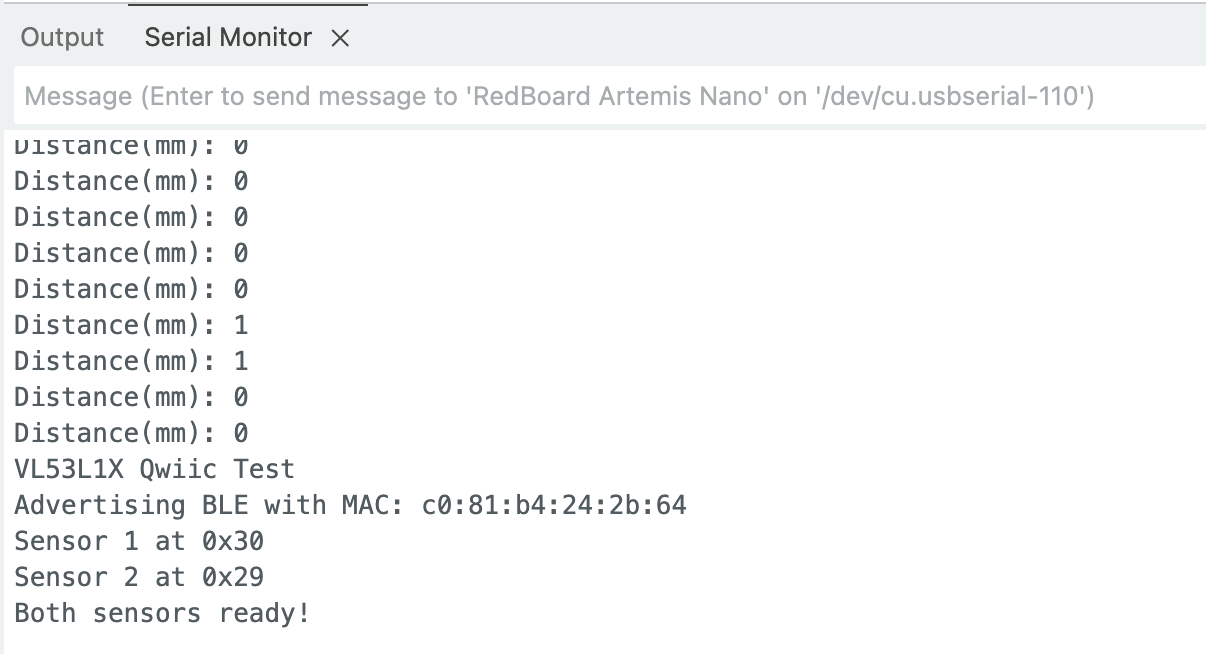
Both ToF sensors reading distances simultaneously over Serial.
I2C Pull-Up Resistors
When using two SparkFun VL53L1X breakout boards on the same I2C bus, both boards include their own I2C pull-up resistors. Two sets of pull-ups in parallel halve the effective resistance, which can violate I2C spec and cause bus communication errors. The recommended fix is to cut the pull-up resistor trace on one board. Since the Qwiic ecosystem uses 3.3V and the Artemis Nano's Qwiic connector includes internal protection circuitry, both sensors communicated reliably without modification in testing — but cutting one board's pull-up traces would be best practice for a permanent robot build.
Task 9: Non-Blocking Loop — Artemis Clock at Full Speed
To prevent the loop from hanging while waiting for sensor data, I use a
non-blocking polling pattern. startRanging() is called once before
the BLE loop begins; each iteration then only checks
checkForDataReady() without any delay().
The Artemis clock (millis()) is printed every iteration regardless
of whether new sensor data is available.
// Non-blocking ranging helpers

void startNonBlockingRanging() {
    sensor1.startRanging();
    sensor2.startRanging();
    sensor1_ranging = true;
    sensor2_ranging = true;
}

void checkAndReadSensors() {
    // Sensor 1 — read only when data is ready
    if (sensor1_ranging && sensor1.checkForDataReady()) {
        distance1 = sensor1.getDistance();
        sensor1.clearInterrupt();
        sensor1.stopRanging();
        sensor1.startRanging();   // restart immediately
    }
    // Sensor 2 — same pattern
    if (sensor2_ranging && sensor2.checkForDataReady()) {
        distance2 = sensor2.getDistance();
        sensor2.clearInterrupt();
        sensor2.stopRanging();
        sensor2.startRanging();
    }
}

// Inside while(central.connected()):
Serial.print("T(ms): ");
Serial.println(millis());   // prints every iteration
checkAndReadSensors();      // only reads when data ready
Loop Speed and Limiting Factor
The Artemis loop runs thousands of iterations per second —
the millis() print and sensor check together execute in
microseconds. The limiting factor is the ToF sensor measurement time,
not the microcontroller. In Long mode, the VL53L1X takes approximately 20 ms per
reading (~50 Hz). The loop prints the clock far more frequently than new distance
data arrives, confirming that the non-blocking approach keeps the processor
fully available between sensor updates.
Task 10: Time-Stamped ToF and IMU Data via BLE
I combined the Lab 2 IMU code (complementary filter for pitch/roll/yaw) with the
Lab 3 dual-ToF code into a single sketch. Two new BLE commands were added:
START_RECORD buffers ToF and IMU data into arrays for 5 seconds;
SEND_RECORD transmits all buffered data over BLE and signals
completion with "DONE".
Arduino Recording Logic
#define MAX_RECORD 500
#define RECORD_DURATION 5000  // ms

// Buffers
int rec_d1[MAX_RECORD], rec_d2[MAX_RECORD];
unsigned long rec_tof_t[MAX_RECORD];
int rec_tof_count = 0;

float rec_compl_pitch[MAX_RECORD], rec_compl_roll[MAX_RECORD], rec_compl_yaw[MAX_RECORD];
unsigned long rec_imu_t[MAX_RECORD];
int rec_imu_count = 0;

// Store ToF sample (inside checkAndReadSensors when recording)
if (recording && rec_tof_count < MAX_RECORD) {
    rec_d1[rec_tof_count]    = distance1;
    rec_d2[rec_tof_count]    = distance2;
    rec_tof_t[rec_tof_count] = millis() - record_start;
    rec_tof_count++;
}

// Store IMU sample (called each loop iteration via recordIMU())
void recordIMU() {
    if (recording && rec_imu_count < MAX_RECORD && myICM.dataReady()) {
        myICM.getAGMT();
        updateAccelPitchRoll();
        updateGyroRollPitchYaw();
        updateComplRollPitchYaw();
        rec_compl_pitch[rec_imu_count] = compl_pitch;
        rec_compl_roll[rec_imu_count]  = compl_roll;
        rec_compl_yaw[rec_imu_count]   = compl_yaw;
        rec_imu_t[rec_imu_count]       = millis() - record_start;
        rec_imu_count++;
    }
}
Python BLE Collection Code
rec_d1, rec_d2, rec_tof_t = [], [], []
rec_pitch, rec_roll, rec_yaw, rec_imu_t = [], [], [], []
done_flag = [False]

def record_notif_handler(uuid, byte_array):
    s = ble.bytearray_to_string(byte_array)
    if s == 'DONE':
        done_flag[0] = True
        return
    parts = s.split(',')
    if parts[0] == 'TOF':
        rec_d1.append(int(parts[1]))
        rec_d2.append(int(parts[2]))
        rec_tof_t.append(int(parts[3]))
    elif parts[0] == 'IMU':
        rec_pitch.append(float(parts[1]))
        rec_roll.append(float(parts[2]))
        rec_yaw.append(float(parts[3]))
        rec_imu_t.append(int(parts[4]))

ble.start_notify(ble.uuid['TX_STRING'], record_notif_handler)
ble.send_command(CMD_lab3.START_RECORD, '')
print('Recording for 5 seconds...')
time.sleep(5.5)
ble.send_command(CMD_lab3.SEND_RECORD, '')
while not done_flag[0]: time.sleep(0.1)
ble.stop_notify(ble.uuid['TX_STRING'])
print(f'ToF: {len(rec_d1)} samples, IMU: {len(rec_pitch)} samples')
Task 11: ToF Data Against Time
After recording, timestamps are converted to seconds (relative to the first sample) and both sensor distances are plotted on the same axes:
t_tof = (np.array(rec_tof_t) - rec_tof_t[0]) / 1000.0

plt.figure()
plt.plot(t_tof, rec_d1, 'b-o', markersize=3, label='Sensor 1 (front)')
plt.plot(t_tof, rec_d2, 'r-o', markersize=3, label='Sensor 2 (side)')
plt.xlabel('Time (s)')
plt.ylabel('Distance (mm)')
plt.title('ToF Distance vs Time (5-second recording)')
plt.legend()
plt.grid(True)
plt.show()
Both sensors sample at approximately 50 Hz in Long mode and are interleaved in the recording buffer by whichever sensor finishes its measurement first.
Task 12: IMU Data Against Time
The IMU stores complementary-filtered pitch, roll, and yaw. The complementary
filter (from Lab 2) blends accelerometer angle estimates with gyroscope
integration using accel_gain = 0.1 (10% accelerometer, 90%
gyroscope), providing both short-term stability and long-term drift correction.
t_imu = (np.array(rec_imu_t) - rec_imu_t[0]) / 1000.0

plt.figure()
plt.plot(t_imu, rec_pitch, color='red',   label='Pitch')
plt.plot(t_imu, rec_roll,  color='blue',  label='Roll')
plt.plot(t_imu, rec_yaw,   color='green', label='Yaw')
plt.xlabel('Time (s)')
plt.ylabel('Angle (°)')
plt.title('IMU Complementary Filter (Pitch / Roll / Yaw) vs Time')
plt.legend()
plt.grid(True)
plt.show()
Yaw integrates the gyroscope only and drifts slowly over time, while pitch and roll are stabilized by the accelerometer correction term. Over a 5-second window the drift is small and acceptable for robot control.
References
- VL53L1X API Manual (UM2356) — ST Microelectronics
- VL53L1X Datasheet — ST Microelectronics
- Lab 3 Instructions — Fast Robots @ Cornell
- SparkFun VL53L1X Arduino Library documentation
- Arduino Wire library documentation (7-bit address convention)
- Aidan Derocher, past student report (for 0x52 → 0x29 address explanation reference)