Lab 2: IMU
Objective
The purpose of this lab is to add the IMU to the robot, run the Artemis and sensors from a battery, and record a stunt on the RC robot. This involves setting up the ICM-20948 IMU, processing accelerometer and gyroscope data, implementing a low-pass filter, and implementing a complementary filter for stable angle estimation.
Prelab
Prior to lab, I read about the IMU we would be putting on our robot, the ICM-20948, and the SparkFun breakout board. I also skimmed the full lab instructions to prepare for the lab session.
Setup the IMU
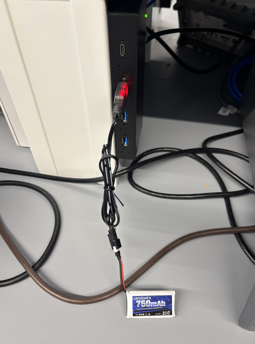
Coming into lab, I exchanged my two puffy 650 mAh batteries (which had been sitting on the shelves too long) for a 750 mAh battery and put it on charge.
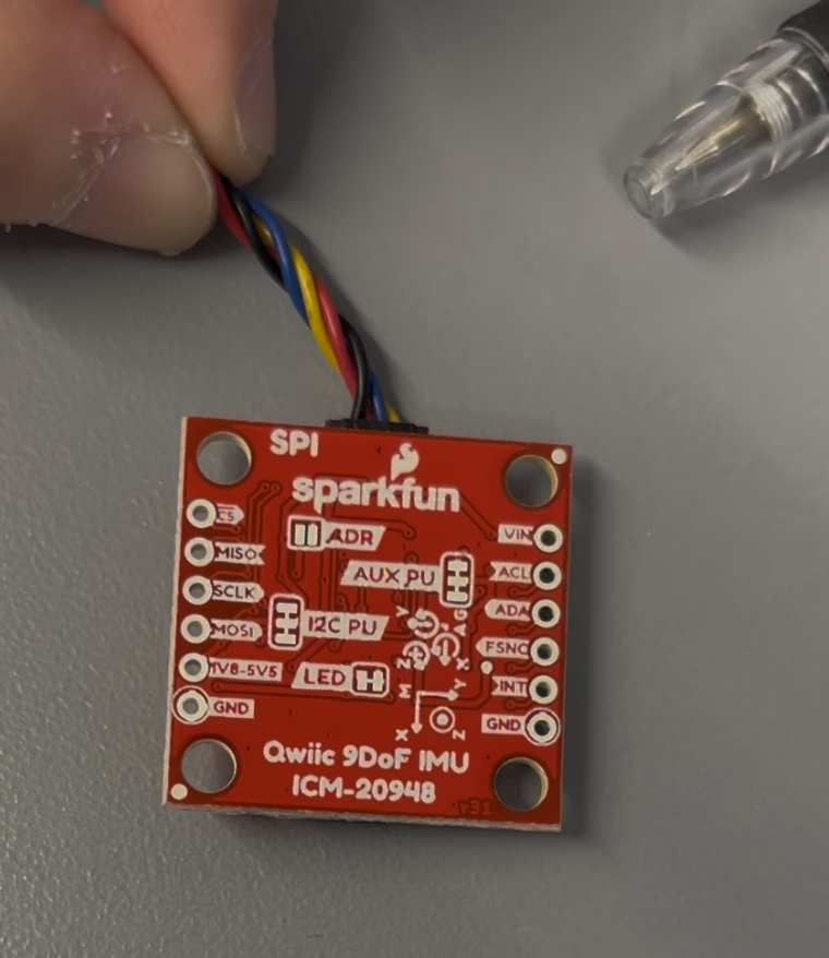
I installed the "SparkFun 9DOF IMU Breakout_ICM 20948_Arduino Library" from the Arduino Library Manager and connected the IMU to the Artemis board using the rainbow-colored QWIIC connectors.
AD0_VAL
I ran the SparkFun ICM-20948 Example1_Basics. The demo code defines AD0_VAL as 1.
AD0_VAL represents the value of the last bit of the I2C address. The AD0 pin on the
ICM-20948 breakout board acts as an address select, allowing two IMUs to share the same I2C bus
without conflict. According to the datasheet, the LSB of the 7-bit I2C address is set by the logic
level on pin AD0: address b1101000 (AD0 = 0, logic low) or b1101001
(AD0 = 1, logic high). The code correctly initializes with AD0_VAL = 1, meaning the
library communicates at address 0x69 (b1101001), with the AD0 pin on the breakout board pulled
high by an onboard pull-up resistor.
Sensor Values: Rotate, Flip, Accelerate
I changed delay(30) to delay(300) to better observe changing values in
the Serial Monitor. As I rotate, flip, and accelerate the board, the accelerometer and gyroscope
data values change accordingly.
When the IMU is placed flat and stationary on the table, the X and Y accelerometer values hover near 0 mg while Z hovers near 1000 mg (~1g). For instance, a typical reading shows X = 21 mg, Y = −17.58 mg, Z = 1026.37 mg, which converts to X = 0.021g, Y = −0.018g, Z = 1.026g. This is expected because gravity acts straight down, so only the Z-axis sees it. The small offsets are sensor noise and minor calibration bias. With the IMU stationary, gyroscope readings are all close to zero (e.g., 1.22 °/s X, 0.80 °/s Y, 0.96 °/s Z).
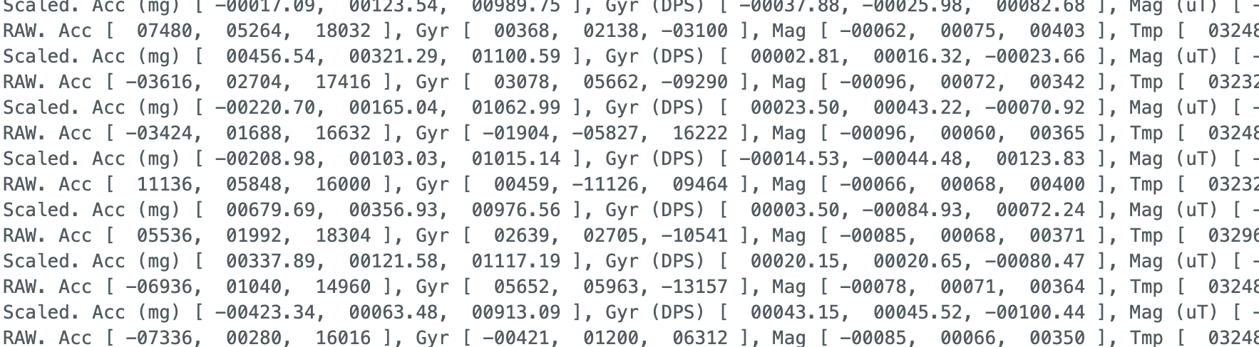
When I rotate the IMU, whichever axis aligns with the rotation has a significantly larger gyroscope value than the other two. For example, rotating around the pitch axis (Y) produces large gyroscope Y readings and large varying accelerometer values because gravity's projection shifts across axes as the board is flipped.
When I push the IMU linearly back and forth in the X direction, the X accelerometer value shifts from positive to negative to positive, reflecting the linear acceleration from my hand. The Y accelerometer is small (I moved primarily along X), and Z stays near 1g. Because I am doing linear, not rotational, motion, the gyroscope readings remain very small.
LED Startup Indication
At startup, an LED blinks slowly 3 times as a visual indication that the board is running.
This is implemented in setup() using digitalWrite and
delay(2000) to create three slow on-off cycles.
// blink LED 3 times slowly on start-up
digitalWrite(LED_BUILTIN, HIGH);
delay(2000);
digitalWrite(LED_BUILTIN, LOW);
delay(2000);
digitalWrite(LED_BUILTIN, HIGH);
delay(2000);
digitalWrite(LED_BUILTIN, LOW);
delay(2000);
digitalWrite(LED_BUILTIN, HIGH);
delay(2000);
digitalWrite(LED_BUILTIN, LOW);
delay(2000);
Accelerometer
Pitch and Roll Equations
Pitch and roll are computed from the raw accelerometer X, Y, Z readings using atan2
and converted from radians to degrees:
void updateAccelPitchRoll() {
  float a_x = myICM.accX();
  float a_y = myICM.accY();
  float a_z = myICM.accZ();
  // atan2 returns radians, convert to degrees
  accel_roll  = atan2(a_y, a_z) * 180.0 / M_PI;
  accel_pitch = atan2(a_x, a_z) * 180.0 / M_PI;
}
This requires including the math.h library for atan2 and M_PI.
Output at {−90°, 0°, 90°} for Pitch and Roll
I used the surface and edges of my table as guides to achieve consistent 90° tilts. The pitch and roll angles were displayed on the Serial Monitor and simultaneously streamed to Python over BLE.
Figure 5 shows the pitch and roll when the IMU is placed flat on the table (expected: pitch ≈ 0°, roll ≈ 0°). The measured pitch is ~0.11° and roll is ~−0.95°, both very close to 0°, confirming the accelerometer is reading correctly at the flat position.
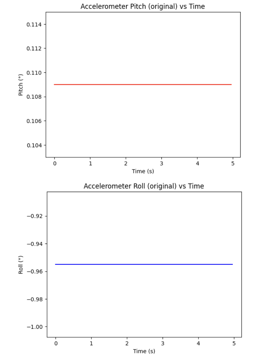
Figure 6 shows the pitch and roll when the IMU is again placed flat — the pitch stays at ~0.11° and roll at ~−0.95°, consistent with Figure 5. This was collected at the desk edge position to prepare for the −90° edge calibration measurement.
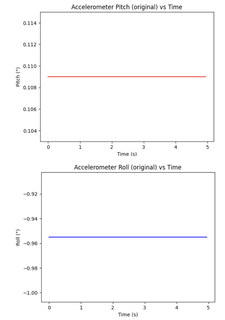
Figure 7 shows pitch and roll at the +90° edge position. Roll reads ~88.2° and pitch reads ~45.9°. The roll is close to the expected 90°, though pitch also shows a compound tilt because achieving a perfectly pure single-axis 90° rotation by hand on the desk edge is difficult.
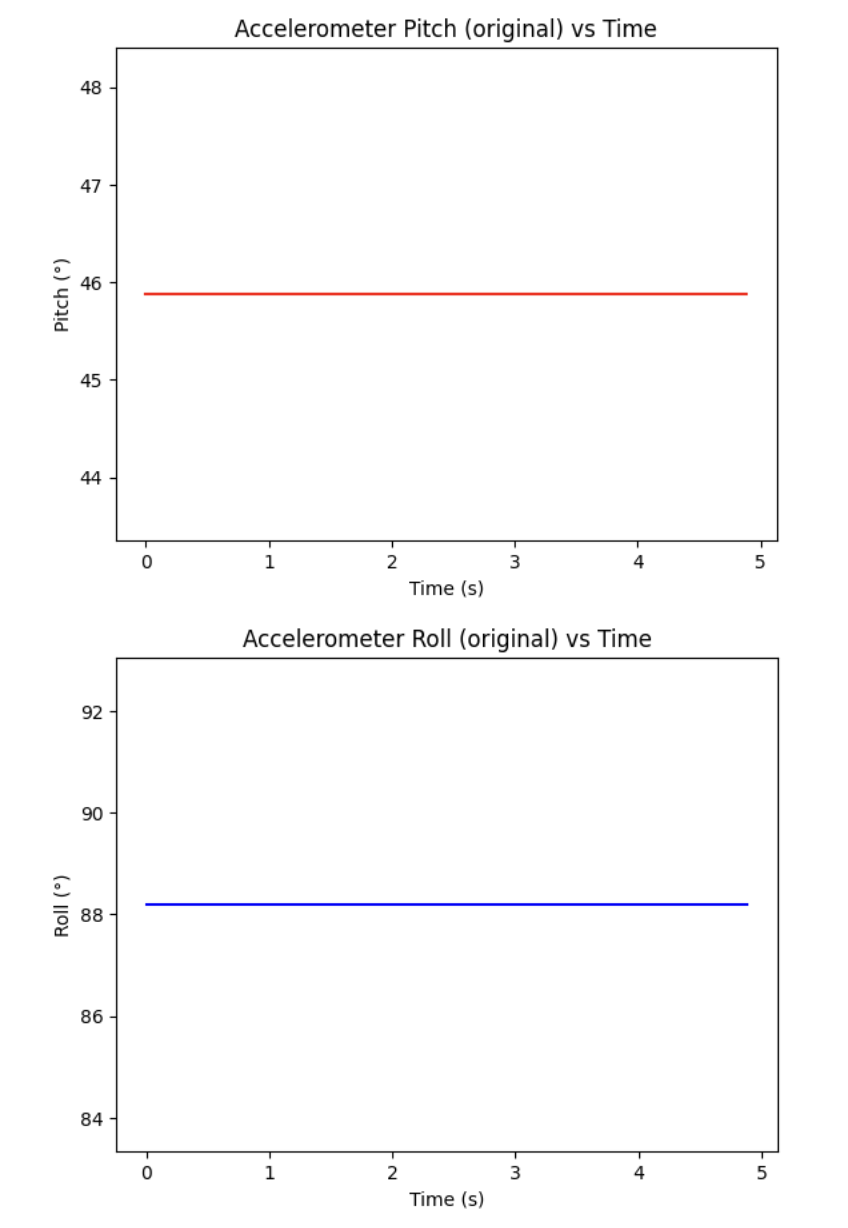
Figure 6 shows the pitch and roll when the IMU is propped on the right edge of my desk (expected: pitch ≈ 0°, roll ≈ −90°). Roll reads ~−0.95°, which is unexpectedly not close to −90°. This is because the IMU was placed on the edge along an axis that changed roll rather than pitch, and the physical alignment was not perfectly perpendicular. This highlights the difficulty of achieving exactly 90° by hand.
Figure 7 shows pitch and roll at +90°. Roll reads ~88.2° and pitch reads ~45.9°, showing that the IMU was not placed at a pure single-axis rotation — it had compound tilt. The table edge provided a reasonable but imperfect guide.
Plotting in Python with BLE
To better process data, I established a BLE connection between the Artemis (Arduino IDE)
and my laptop (Jupyter Lab). I combined the BLE communication code into lab2_imu.ino,
adding the required libraries, UUIDs, and case statements for commands including
GET_ACCEL_DATA, GET_ACCEL_NOISE, GET_GYRO_DATA, and
GET_COMPL_DATA. When I first compiled after combining everything, I got a
redefinition error because both files defined handle_command() and read_data().
handle_command() and read_data() when first combining ble_arduino.ino with lab2_imu.ino. Resolved by merging into a single sketch folder with copied header files.
ble_arduino.ino and lab2_imu.ino. Resolved by copying header files into the lab2_imu sketch folder.Accelerometer Accuracy and Two-Point Calibration
To assess accuracy, I performed a two-point calibration by measuring pitch and roll at +90°
and −90°. The mean values at each orientation were collected using np.mean() in Python:
- At +90°: mean pitch = 45.881°, mean roll = 88.197°
- At −90°: mean pitch = −2.385°, mean roll = −88.026°
A note on the calibration process: every time I aligned the IMU next to my desk's edge for a more accurate 90°, the IMU would disconnect due to physical contact with the edge, which was frustrating and limited calibration accuracy.
The scale and offset were computed as follows:
# take the mean at +90°
mean_pitch_90_measured  = np.mean(accel_pitches)
mean_roll_90_measured   = np.mean(accel_rolls)

# take the mean at -90°
mean_pitch_neg_90_measured = np.mean(accel_pitches)
mean_roll_neg_90_measured  = np.mean(accel_rolls)

# compute scale and offset
pitch_scale  = 180.0 / (mean_pitch_90_measured - mean_pitch_neg_90_measured)
pitch_offset = 90.0  - pitch_scale * mean_pitch_90_measured
roll_scale   = 180.0 / (mean_roll_90_measured  - mean_roll_neg_90_measured)
roll_offset  = 90.0  - roll_scale  * mean_roll_90_measured
The resulting conversion factors are:
- Pitch scale: 1.0224, Pitch offset: −0.9508°
- Roll scale: 0.9965, Roll offset: −0.8819°
Pitch scale is ~1.02 (2% off from ideal) and roll scale is ~1.00 (very close to ideal), with small offsets. This indicates the ICM-20948 accelerometer is quite accurate and calibration provides only a small correction.
Noise in the Frequency Spectrum
To analyze accelerometer noise, I implemented a GET_ACCEL_NOISE BLE command that
records 100 samples at ~200 Hz (5 ms delay between samples) into arrays on the Artemis, then
sends them all over BLE. This store-then-send approach ensures consistent sampling without BLE
transmission overhead disturbing the timing.
// Arduino: GET_ACCEL_NOISE — store first, then send
case GET_ACCEL_NOISE:
  for (int i = 0; i < ARRAY_SIZE; i++) {
    if (myICM.dataReady()) {
      myICM.getAGMT();
      updateAccelPitchRoll();
      accel_pitch_arr[i] = accel_pitch;
      accel_roll_arr[i]  = accel_roll;
      arr[i] = millis();
    }
    delay(5); // 5ms = ~200Hz
  }
  for (int i = 0; i < ARRAY_SIZE; i++) {
    tx_estring_value.clear();
    tx_estring_value.append("Accel_pitch:"); tx_estring_value.append(accel_pitch_arr[i]);
    tx_estring_value.append(",Accel_roll:"); tx_estring_value.append(accel_roll_arr[i]);
    tx_estring_value.append(",T:");          tx_estring_value.append((int)arr[i]);
    tx_characteristic_string.writeValue(tx_estring_value.c_str());
    delay(10);
  }
# Python: collect noise data
noise_timestamps = []; noise_pitches = []; noise_rolls = []
def accel_noise_notif_handler(uuid, byte_array):
s = ble.bytearray_to_string(byte_array)
s_split = dict(item.split(":") for item in s.split(","))
noise_pitches.append(float(s_split["Accel_pitch"]))
noise_rolls.append(float(s_split["Accel_roll"]))
noise_timestamps.append(int(s_split["T"]))
noise_timestamps.clear(); noise_pitches.clear(); noise_rolls.clear()
ble.start_notify(ble.uuid['RX_STRING'], accel_noise_notif_handler)
ble.send_command(CMD_lab2.GET_ACCEL_NOISE, "")
time.sleep(4)
ble.stop_notify(ble.uuid['RX_STRING'])
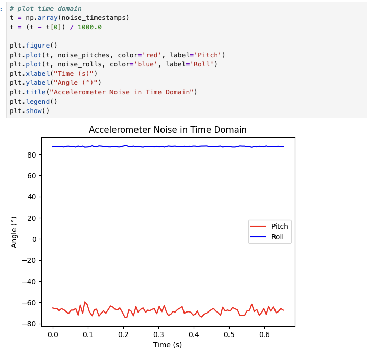
print(f"Collected {len(noise_timestamps)}/100 samples")Figure 9 shows the noise in the time domain with the IMU held at an angled position (~−65° pitch, ~88° roll). The pitch signal (red) has visible noise oscillations of roughly ±5°, while the roll signal (blue) is much more stable with smaller oscillations. The overall pattern shows that the accelerometer is sensitive to small vibrations, especially at non-flat orientations where cross-axis coupling is greater.
# Python: FFT using scipy
from scipy.fftpack import fft

def plot_fft(timestamps_ms, signal, color, label):
    N  = len(signal)
    t  = np.array(timestamps_ms)
    dt = np.mean(np.diff(t)) / 1000.0   # ms -> seconds
    fs = 1.0 / dt
    print(f"{label} sampling rate: {fs:.1f} Hz")

    signal = np.array(signal) - np.mean(signal)  # remove DC offset
    freq_data = fft(signal)
    frequency = np.linspace(0, fs/2, N//2)
    y = 2/N * np.abs(freq_data[0:N//2])

    plt.figure()
    plt.plot(frequency, y, color=color)
    plt.xlabel("Frequency (Hz)"); plt.ylabel("Amplitude")
    plt.title(f"FFT - Accelerometer {label}")
    plt.grid(True); plt.show()
    return frequency, y

pitch_freq, pitch_mag = plot_fft(noise_timestamps, noise_pitches, "red",  "Pitch_noise")
roll_freq,  roll_mag  = plot_fft(noise_timestamps, noise_rolls,   "blue", "Roll_noise")
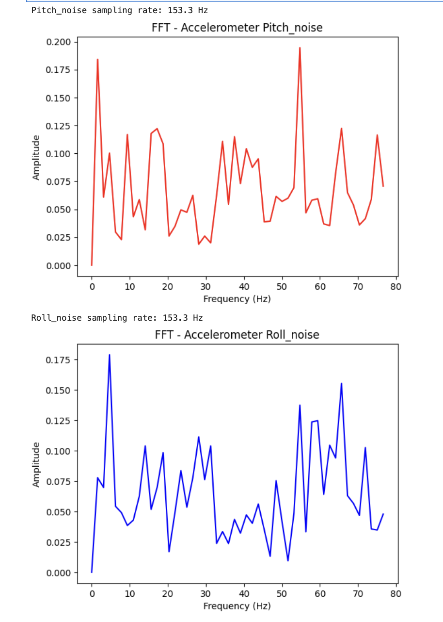
Figure 10 shows the FFT of the pitch and roll noise using scipy.fftpack.fft.
The spectrum is relatively flat across all frequencies from 0 to 76 Hz (Nyquist limit at
153 Hz sampling), with no single dominant spike — characteristic of broadband white noise.
A peak near 0 Hz is the DC component (the mean angle), which was subtracted before computing
the FFT. A spike at approximately 55 Hz is visible in the pitch spectrum; this may correspond
to table vibration, electrical interference, or a spectral artifact from the limited 100-sample
window.
Low-Pass Filter Cutoff Frequency
Since the FFT shows broadband noise distributed across all frequencies with no clear knee point, the cutoff frequency must be chosen based on the expected signal content rather than a visible spectral transition. Real robot motion (tilting, turning) occurs at frequencies below approximately 5 Hz, while noise occupies the full spectrum up to Nyquist. A cutoff frequency of fc = 5 Hz was chosen to pass the meaningful motion signal and reject the higher-frequency noise floor.
The corresponding alpha (accel_gain) for the low-pass filter at 153 Hz sampling (dt = 1/153 s):
alpha = (2π × fc × dt) / (2π × fc × dt + 1)
      = (2π × 5 × 0.0065) / (2π × 5 × 0.0065 + 1)
      ≈ 0.17
A lower cutoff (smaller alpha) produces a smoother output with more lag, which is preferable for the IMU use case since we want stable angle estimates for the PID controller rather than raw noisy readings. A higher cutoff (larger alpha) passes more noise but is more responsive.
Low-Pass Filter Implementation
The low-pass filter is implemented on the Artemis in the GET_ACCEL_DATA case:
// Arduino: GET_ACCEL_DATA with LPF
case GET_ACCEL_DATA:
  updateAccelPitchRoll();
  // lpf: angle_lpf = alpha*angle + (1-alpha)*angle_lpf_prev
  accel_roll_lpf  = accel_gain * accel_roll  + gyro_gain * accel_roll_lpf;
  accel_pitch_lpf = accel_gain * accel_pitch + gyro_gain * accel_pitch_lpf;

  tx_estring_value.clear();
  tx_estring_value.append("Accel_pitch:");     tx_estring_value.append(accel_pitch);
  tx_estring_value.append(",Accel_roll:");     tx_estring_value.append(accel_roll);
  tx_estring_value.append(",Accel_roll_lpf:"); tx_estring_value.append(accel_roll_lpf);
  tx_estring_value.append(",Accel_pitch_lpf:"); tx_estring_value.append(accel_pitch_lpf);
  tx_estring_value.append(",T:");              tx_estring_value.append((int)millis());
  tx_characteristic_string.writeValue(tx_estring_value.c_str());
  break;
where accel_gain = 0.17 (alpha) and gyro_gain = 1 - accel_gain = 0.83.
The LPF globals are initialized at the end of setup() to the first IMU reading
to avoid the exponential convergence artifact from zero initialization:
// Arduino: setup() — initialize LPF to first real reading
myICM.getAGMT();
updateAccelPitchRoll();
accel_roll_lpf  = accel_roll;
accel_pitch_lpf = accel_pitch;
# Python: collect and plot accel raw vs LPF
timestamps = []; accel_pitches = []; accel_rolls = []
accel_pitches_lpf = []; accel_rolls_lpf = []
def accel_reading_notif_handler(uuid, byte_array):
s = ble.bytearray_to_string(byte_array)
parts = dict(item.split(":") for item in s.split(","))
accel_pitches.append(float(parts["Accel_pitch"]))
accel_rolls.append(float(parts["Accel_roll"]))
accel_pitches_lpf.append(float(parts["Accel_pitch_lpf"]))
accel_rolls_lpf.append(float(parts["Accel_roll_lpf"]))
timestamps.append(int(parts["T"]))
timestamps.clear(); accel_pitches.clear(); accel_rolls.clear()
accel_pitches_lpf.clear(); accel_rolls_lpf.clear()
ble.start_notify(ble.uuid['RX_STRING'], accel_reading_notif_handler)
t_start = time.time()
while time.time() - t_start < 5:
ble.send_command(CMD_lab2.GET_ACCEL_DATA, "")
time.sleep(0.05)
print(f"Collected {len(timestamps)} samples in 5 seconds")
ble.stop_notify(ble.uuid['RX_STRING'])
Figure 11 shows the LPF output exhibiting an initialization artifact — the LPF starts far from
the true angle and exponentially converges to it over several seconds. This occurred because
accel_pitch_lpf was initialized to 0 rather than to the first real sensor reading.
This was fixed by initializing the LPF variables at the end of setup() to the
actual first IMU reading:
// Arduino: setup() — initialize LPF to first real reading to avoid artifact
myICM.getAGMT();
updateAccelPitchRoll();
accel_roll_lpf  = accel_roll;
accel_pitch_lpf = accel_pitch;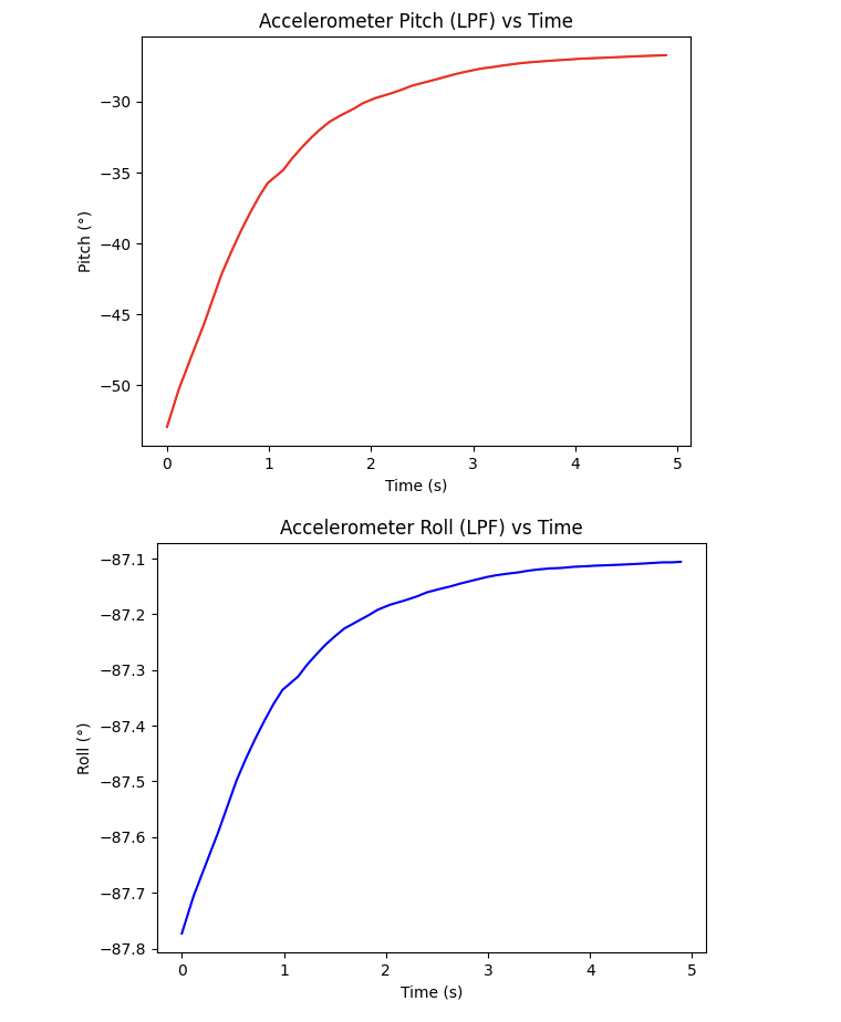
setup().Gyroscope
Pitch, Roll, and Yaw from Gyroscope
Gyroscope pitch, roll, and yaw are computed by integrating the angular velocity readings over time using the following equations:
gyro_roll  += gyrX() * dt;
gyro_pitch += gyrY() * dt;
gyro_yaw   += gyrZ() * dt;
where dt is the actual elapsed time since the last measurement, computed
dynamically using millis():
// Arduino: dynamic dt gyroscope integration
void updateGyroRollPitchYaw() {
  unsigned long now = millis();
  dt = (now - last_time) / 1000.0;  // ms -> seconds
  last_time = now;
  gyro_roll  += myICM.gyrX() * dt;
  gyro_pitch += myICM.gyrY() * dt;
  gyro_yaw   += myICM.gyrZ() * dt;
}
Originally, dt was hardcoded as 0.001 s, which was incorrect because the main
loop runs at ~300 ms (not 1 ms). Using dynamic dt based on actual timestamps
produces accurate angle integration.
# Python: collect gyroscope data
gyro_timestamps = []; gyro_pitches = []; gyro_rolls = []; gyro_yaws = []

def gyro_reading_notif_handler(uuid, byte_array):
    s = ble.bytearray_to_string(byte_array)
    parts = dict(item.split(":") for item in s.split(","))
    gyro_pitches.append(float(parts["Gyro_pitch"]))
    gyro_rolls.append(float(parts["Gyro_roll"]))
    gyro_yaws.append(float(parts["Gyro_yaw"]))
    gyro_timestamps.append(int(parts["T"]))

gyro_timestamps.clear(); gyro_pitches.clear()
gyro_rolls.clear(); gyro_yaws.clear()

ble.start_notify(ble.uuid['RX_STRING'], gyro_reading_notif_handler)
DURATION = 5
SAMPLE_DELAY = 0.05  # change to adjust sampling frequency
t_start = time.time()
while time.time() - t_start < DURATION:
    ble.send_command(CMD_lab2.GET_GYRO_DATA, "")
    time.sleep(SAMPLE_DELAY)
print(f"Collected {len(gyro_timestamps)} samples in {DURATION}s")
Comparison to Accelerometer and Filtered Response
The three sensing approaches differ in the following key ways:
- Accelerometer (raw): Noisy but accurate in the long run. The mean of the noise has a zero Gaussian offset, meaning it returns to the correct absolute angle over time. However, the accelerometer cannot measure yaw because yaw is rotation around the vertical (gravity) axis — gravity has no component that changes with yaw rotation, so atan2 cannot recover it.
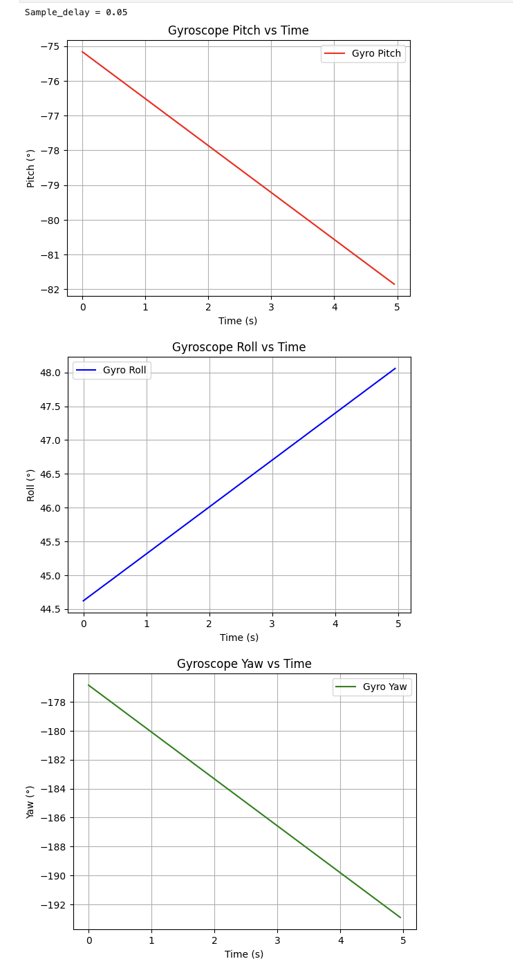
- Gyroscope: Smooth and responsive, but suffers from drift — integrating even a tiny bias in angular velocity causes the angle to slowly wander over time even when the IMU is stationary, as shown in Figures 13 and 14. The gyroscope can measure yaw, but drift affects yaw too.
- Low-pass filtered accelerometer: Smoother than raw accelerometer with reduced high-frequency noise, but still cannot measure yaw and still contains the accelerometer's susceptibility to linear vibrations.
Effect of Sampling Frequency on Gyroscope Accuracy
Sampling frequency directly affects the accuracy of gyroscope angle integration. With a slower
sampling rate (larger delay()), each integration step is larger, meaning even a small
gyroscope bias accumulates into a larger error per step. Figure 14 shows gyroscope data collected
at sample_delay = 0.05 s (approximately 20 Hz) — the drift is steeper and more
visible than at higher sampling rates (e.g., delay(10) at ~100 Hz). At faster
sampling, each dt is smaller so bias accumulates more slowly.
Yes — adjusting sampling frequency here means changing dt (the time between
measurements), which is controlled by the delay() in the main loop. A smaller
delay means more frequent updates, smaller dt, and less drift accumulation.
Complementary Filter
The complementary filter combines the gyroscope (short-term accuracy, no vibration sensitivity) with the accelerometer (long-term accuracy, no drift) to produce an estimate that is both stable and accurate:
compl_roll  = gyro_gain  * (compl_roll  + gyrX() * dt) + accel_gain * accel_roll;
compl_pitch = gyro_gain  * (compl_pitch + gyrY() * dt) + accel_gain * accel_pitch;
compl_yaw   = gyro_yaw;  // no accelerometer correction for yaw
// Arduino: complementary filter
void updateComplRollPitchYaw() {
compl_roll = gyro_gain * (compl_roll + myICM.gyrX() * dt) + accel_gain * accel_roll;
compl_pitch = gyro_gain * (compl_pitch + myICM.gyrY() * dt) + accel_gain * accel_pitch;
compl_yaw = gyro_yaw; // no accelerometer correction for yaw
}
// globals
float accel_gain = 0.1; // 10% accel, 90% gyro
float gyro_gain = 1.0 - accel_gain;# Python: collect complementary filter data and overlay plot
compl_timestamps = []; compl_pitches = []; compl_rolls = []; compl_yaws = []
def compl_notif_handler(uuid, byte_array):
s = ble.bytearray_to_string(byte_array)
parts = dict(item.split(":") for item in s.split(","))
compl_pitches.append(float(parts["Compl_pitch"]))
compl_rolls.append(float(parts["Compl_roll"]))
compl_yaws.append(float(parts["Compl_yaw"]))
compl_timestamps.append(int(parts["T"]))
compl_timestamps.clear(); compl_pitches.clear()
compl_rolls.clear(); compl_yaws.clear()
ble.start_notify(ble.uuid['RX_STRING'], compl_notif_handler)
t_start = time.time()
while time.time() - t_start < 5:
ble.send_command(CMD_lab2.GET_COMPL_DATA, "")
time.sleep(0.05)
# overlay accel vs gyro vs complementary
t_c = (np.array(compl_timestamps) - compl_timestamps[0]) / 1000.0
t_a = (np.array(timestamps) - timestamps[0]) / 1000.0
t_g = (np.array(gyro_timestamps) - gyro_timestamps[0]) / 1000.0
plt.figure()
plt.plot(t_a, accel_pitches, color='blue', alpha=0.5, label='Accel (raw)')
plt.plot(t_g, gyro_pitches, color='green', alpha=0.5, label='Gyro')
plt.plot(t_c, compl_pitches, color='red', linewidth=2, label='Complementary')
plt.xlabel("Time (s)"); plt.ylabel("Pitch (°)")
plt.title("Pitch: Accel vs Gyro vs Complementary Filter")
plt.legend(); plt.grid(True); plt.show()
With accel_gain = 0.5 and gyro_gain = 0.5, the filter heavily weights
the accelerometer and the complementary output closely tracks the raw accelerometer value.
Reducing accel_gain to 0.1 (trusting the gyroscope 90%) makes the complementary
filter more responsive while still receiving long-term correction from the accelerometer,
as seen in Figure 15 where the complementary filter (red) stays close to the accel (blue)
while the gyroscope (green) drifts away.
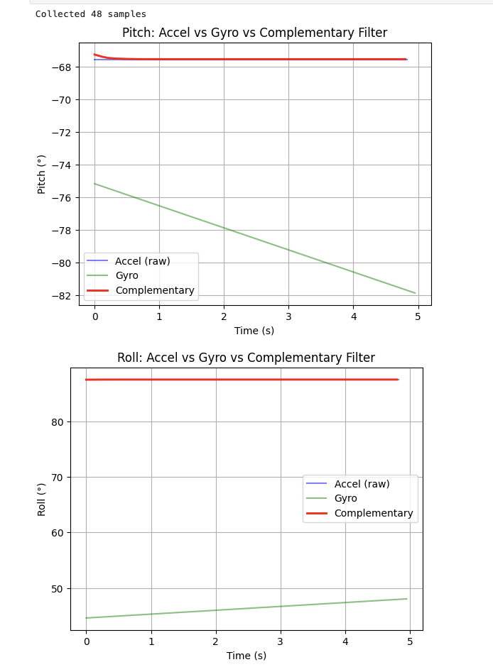
The complementary filter demonstrates its value clearly: the gyroscope drifts several degrees over 5 seconds while the complementary filter remains anchored to the true angle. The filter is also not susceptible to quick vibrations because the gyroscope component smooths out the high-frequency accelerometer spikes, and the accelerometer component corrects the long-term gyroscope drift.
Sample Data
Speeding Up the Main Loop
To maximize sampling speed, I made the following changes to the main loop:
// Arduino: non-blocking main loop
void loop() {
  BLEDevice central = BLE.central();
  if (central) {
    while (central.connected()) {
      write_data();
      read_data();  // handles BLE commands
    }
  }
  // non-blocking IMU check — no delay(), no Serial.print()
  if (myICM.dataReady()) {
    myICM.getAGMT();
    updateAccelPitchRoll();
    updateGyroRollPitchYaw();  // must be called first — updates dt
    updateComplRollPitchYaw(); // depends on dt from above
    delay(10); // ~100Hz
  }
}-
Removed
delay(300)from the main loop and replaced it with a non-blockingif (myICM.dataReady())check. This means the loop does not wait for IMU data to be ready — it simply checks and moves on if data is not yet available. -
Removed all
Serial.printstatements, which are a significant source of delays due to UART transmission overhead. - Removed debugging delays.
The ICM-20948's default output data rate (ODR) is approximately 1125 Hz / (1 + SMPLRT_DIV).
With default settings, the IMU produces new values at roughly 100–200 Hz. The Artemis main loop
without delays runs much faster than this, so the loop will frequently find
dataReady() == false and skip the IMU block — meaning the loop runs faster than
the IMU produces values. This is the correct behavior: the loop polls rapidly and processes
data only when new data is available.
Data Storage Design
I use separate arrays for accelerometer and gyroscope data rather than one large interleaved array. This is because the two sensors may be sampled at different effective rates (the IMU produces both at the same time, but future labs may require streaming only one), and separate arrays make the code easier to read, debug, and extend. A shared timestamp array is used for both.
I use floats (4 bytes each) for angle data. Double precision is unnecessary for angle measurements in this application (float gives ~7 decimal digits of precision, more than sufficient). Integer storage would lose the fractional part of the angle. Strings consume significantly more memory and require conversion overhead.
The Artemis has 384 kB of RAM. Accounting for program code, BLE stack, and other variables, a conservative estimate of ~200 kB is available for data arrays. With 3 float arrays (pitch, roll, yaw) plus 1 unsigned long timestamp array, each sample costs 3 × 4 + 4 = 16 bytes. This allows approximately 200,000 / 16 ≈ 12,500 samples. At a sampling rate of ~150 Hz, that corresponds to roughly 83 seconds of data storage.
5 Seconds of IMU Data over Bluetooth
Using the GET_ACCEL_DATA and GET_GYRO_DATA BLE commands with a
Python collection loop running for 5 seconds, the board successfully captures and transmits
time-stamped IMU data over Bluetooth.
Recording a Stunt
I mounted the 750 mAh battery in the RC car (red to red, black to black) and installed 2 AA batteries in the remote controller. I spent time driving the car in the hallway to get a feel for its behavior.
Observations from driving the RC car:
- The car is fast — it accelerates very quickly from a stop and reaches a high top speed in a short distance. This will produce significant IMU acceleration spikes when the motors are engaged.
- Turning is sharp. At full throttle, the car can spin nearly in place. Sharp turns also produce visible roll on the chassis.
- The car can drive forward and backward with similar speed. Rapid direction changes (forward to reverse) cause the car to jerk abruptly.
- Motor vibrations are noticeable when the car runs nearby — this confirms that the accelerometer noise analysis is important for future control loops, as the motors will induce high-frequency vibrations into the IMU signal.
- To do a flip, I have to run the car into a wall.
References
- ICM-20948 Datasheet
- Fourier Transform in Python – AlphaBOLD
- Lab 2 Instructions – Fast Robots @ Cornell
- I didn't reference past student's page for this lab.